Perhaps the most ingenious technique was that of the delay line. A delay line is any kind of device which delays the propagation of a pulse or wave signal. If you've ever heard a sound echo back and forth through a canyon or cave, you've experienced an audio delay line: the noise wave travels at the speed of sound, bouncing off of walls and reversing direction of travel. The delay line "stores" data on a very temporary basis if the signal is not strengthened periodically, but the very fact that it stores data at all is a phenomenon exploitable for memory technology.

Early computer delay lines used long tubes filled with liquid mercury, which was used as the physical medium through which sound waves traveled along the length of the tube. An electrical/sound transducer was mounted at each end, one to create sound waves from electrical impulses, and the other to generate electrical impulses from sound waves. A stream of serial binary data was sent to the transmitting transducer as a voltage signal. The sequence of sound waves would travel from left to right through the mercury in the tube and be received by the transducer at the other end. The receiving transducer would receive the pulses in the same order as they were transmitted:

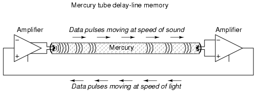
A feedback circuit connected to the receiving transducer would drive the transmitting transducer again, sending the same sequence of pulses through the tube as sound waves, storing the data as long as the feedback circuit continued to function. The delay line functioned like a first-in-first-out (FIFO) shift register, and external feedback turned that shift register behavior into a ring counter, cycling the bits around indefinitely.

The delay line concept suffered numerous limitations from the materials and technology that were then available. The EDVAC computer of the early 1950's used 128 mercury-filled tubes, each one about 5 feet long and storing a maximum of 384 bits. Temperature changes would affect the speed of sound in the mercury, thus skewing the time delay in each tube and causing timing problems. Later designs replaced the liquid mercury medium with solid rods of glass, quartz, or special metal that delayed torsional (twisting) waves rather than longitudinal (lengthwise) waves, and operated at much higher frequencies.

One such delay line used a special nickel-iron-titanium wire (chosen for its good temperature stability) about 95 feet in length, coiled to reduce the overall package size. The total delay time from one end of the wire to the other was about 9.8 milliseconds, and the highest practical clock frequency was 1 MHz. This meant that approximately 9800 bits of data could be stored in the delay line wire at any given time. Given different means of delaying signals which wouldn't be so susceptible to environmental variables (such as serial pulses of light within a long optical fiber), this approach might someday find re-application.

Another approach experimented with by early computer engineers was the use of a cathode ray tube (CRT), the type commonly used for oscilloscope, radar, and television viewscreens, to store binary data. Normally, the focused and directed electron beam in a CRT would be used to make bits of phosphor chemical on the inside of the tube glow, thus producing a viewable image on the screen. In this application, however, the desired result was the creation of an electric charge on the glass of the screen by the impact of the electron beam, which would then be detected by a metal grid placed directly in front of the CRT. Like the delay line, the so-called Williams Tube memory needed to be periodically refreshed with external circuitry to retain its data. Unlike the delay line mechanisms, it was virtually immune to the environmental factors of temperature and vibration. The IBM model 701 computer sported a Williams Tube memory with 4 Kilobyte capacity and a bad habit of "overcharging" bits on the tube screen with successive re-writes so that false "1" states might overflow to adjacent spots on the screen.

The next major advance in computer memory came when engineers turned to magnetic materials as a means of storing binary data. It was discovered that certain compounds of iron, namely "ferrite," possessed hysteresis curves that were almost square:

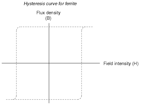
Shown on a graph with the strength of the applied magnetic field on the horizontal axis (field intensity), and the actual magnetization (orientation of electron spins in the ferrite material) on the vertical axis (flux density), ferrite won't become magnetized one direction until the applied field exceeds a critical threshold value. Once that critical value is exceeded, the electrons in the ferrite "snap" into magnetic alignment and the ferrite becomes magnetized. If the applied field is then turned off, the ferrite maintains full magnetism. To magnetize the ferrite in the other direction (polarity), the applied magnetic field must exceed the critical value in the opposite direction. Once that critical value is exceeded, the electrons in the ferrite "snap" into magnetic alignment in the opposite direction. Once again, if the applied field is then turned off, the ferrite maintains full magnetism. To put it simply, the magnetization of a piece of ferrite is "bistable."

Exploiting this strange property of ferrite, we can use this natural magnetic "latch" to store a binary bit of data. To set or reset this "latch," we can use electric current through a wire or coil to generate the necessary magnetic field, which will then be applied to the ferrite. Jay Forrester of MIT applied this principle in inventing the magnetic "core" memory, which became the dominant computer memory technology during the 1970's.

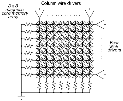
A grid of wires, electrically insulated from one another, crossed through the center of many ferrite rings, each of which being called a "core." As DC current moved through any wire from the power supply to ground, a circular magnetic field was generated around that energized wire. The resistor values were set so that the amount of current at the regulated power supply voltage would produce slightly more than 1/2 the critical magnetic field strength needed to magnetize any one of the ferrite rings. Therefore, if column #4 wire was energized, all the cores on that column would be subjected to the magnetic field from that one wire, but it would not be strong enough to change the magnetization of any of those cores. However, if column #4 wire and row #5 wire were both energized, the core at that intersection of column #4 and row #5 would be subjected to a sum of those two magnetic fields: a magnitude strong enough to "set" or "reset" the magnetization of that core. In other words, each core was addressed by the intersection of row and column. The distinction between "set" and "reset" was the direction of the core's magnetic polarity, and that bit value of data would be determined by the polarity of the voltages (with respect to ground) that the row and column wires would be energized with.

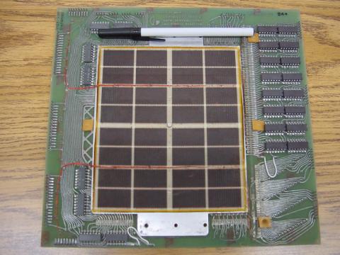
The following photograph shows a core memory board from a Data General brand, "Nova" model computer, circa late 1960's or early 1970's. It had a total storage capacity of 4 kbytes (that's kilobytes, not megabytes!). A ball-point pen is shown for size comparison:

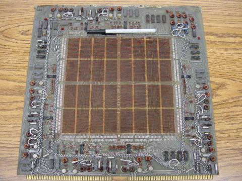
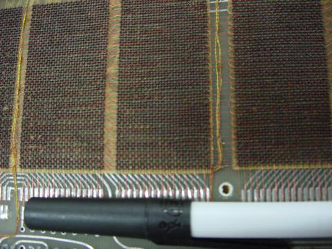
The electronic components seen around the periphery of this board are used for "driving" the column and row wires with current, and also to read the status of a core. A close-up photograph reveals the ring-shaped cores, through which the matrix wires thread. Again, a ball-point pen is shown for size comparison:

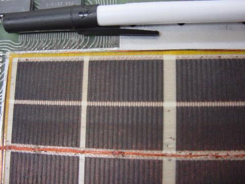
A core memory board of later design (circa 1971) is shown in the next photograph. Its cores are much smaller and more densely packed, giving more memory storage capacity than the former board (8 kbytes instead of 4 kbytes):

And, another close-up of the cores:

Writing data to core memory was easy enough, but reading that data was a bit of a trick. To facilitate this essential function, a "read" wire was threaded through all the cores in a memory matrix, one end of it being grounded and the other end connected to an amplifier circuit. A pulse of voltage would be generated on this "read" wire if the addressed core changed states (from 0 to 1, or 1 to 0). In other words, to read a core's value, you had to write either a 1 or a 0 to that core and monitor the voltage induced on the read wire to see if the core changed. Obviously, if the core's state was changed, you would have to re-set it back to its original state, or else the data would have been lost. This process is known as a destructive read, because data may be changed (destroyed) as it is read. Thus, refreshing is necessary with core memory, although not in every case (that is, in the case of the core's state not changing when either a 1 or a 0 was written to it).

One major advantage of core memory over delay lines and Williams Tubes was nonvolatility. The ferrite cores maintained their magnetization indefinitely, with no power or refreshing required. It was also relatively easy to build, denser, and physically more rugged than any of its predecessors. Core memory was used from the 1960's until the late 1970's in many computer systems, including the computers used for the Apollo space program, CNC machine tool control computers, business ("mainframe") computers, and industrial control systems. Despite the fact that core memory is long obsolete, the term "core" is still used sometimes with reference to a computer's RAM memory.

All the while that delay lines, Williams Tube, and core memory technologies were being invented, the simple static RAM was being improved with smaller active component (vacuum tube or transistor) technology. Static RAM was never totally eclipsed by its competitors: even the old ENIAC computer of the 1950's used vacuum tube ring-counter circuitry for data registers and computation. Eventually though, smaller and smaller scale IC chip manufacturing technology gave transistors the practical edge over other technologies, and core memory became a museum piece in the 1980's.

One last attempt at a magnetic memory better than core was the bubble memory. Bubble memory took advantage of a peculiar phenomenon in a mineral called garnet, which, when arranged in a thin film and exposed to a constant magnetic field perpendicular to the film, supported tiny regions of oppositely-magnetized "bubbles" that could be nudged along the film by prodding with other external magnetic fields. "Tracks" could be laid on the garnet to focus the movement of the bubbles by depositing magnetic material on the surface of the film. A continuous track was formed on the garnet which gave the bubbles a long loop in which to travel, and motive force was applied to the bubbles with a pair of wire coils wrapped around the garnet and energized with a 2-phase voltage. Bubbles could be created or destroyed with a tiny coil of wire strategically placed in the bubbles' path.

The presence of a bubble represented a binary "1" and the absence of a bubble represented a binary "0." Data could be read and written in this chain of moving magnetic bubbles as they passed by the tiny coil of wire, much the same as the read/write "head" in a cassette tape player, reading the magnetization of the tape as it moves. Like core memory, bubble memory was nonvolatile: a permanent magnet supplied the necessary background field needed to support the bubbles when the power was turned off. Unlike core memory, however, bubble memory had phenomenal storage density: millions of bits could be stored on a chip of garnet only a couple of square inches in size. What killed bubble memory as a viable alternative to static and dynamic RAM was its slow, sequential data access. Being nothing more than an incredibly long serial shift register (ring counter), access to any particular portion of data in the serial string could be quite slow compared to other memory technologies.

An electrostatic equivalent of the bubble memory is the Charge-Coupled Device (CCD) memory, an adaptation of the CCD devices used in digital photography. Like bubble memory, the bits are serially shifted along channels on the substrate material by clock pulses. Unlike bubble memory, the electrostatic charges decay and must be refreshed. CCD memory is therefore volatile, with high storage density and sequential access. Interesting, isn't it? The old Williams Tube memory was adapted from CRT viewing technology, and CCD memory from video recording technology.