Δ-Y and Y-Δ conversions

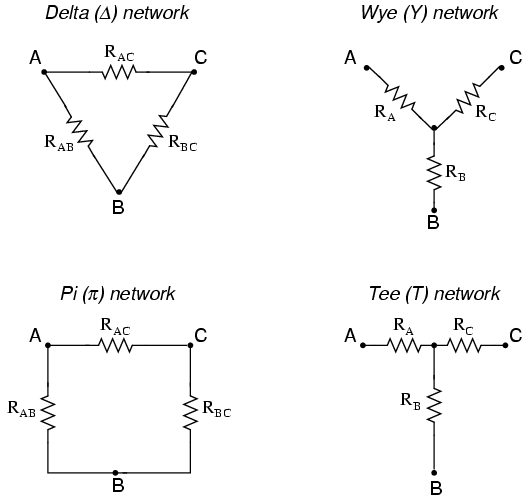
In many circuit applications, we encounter components connected together in one of two ways to form a three-terminal network: the "Delta," or Δ (also known as the "Pi," or π) configuration, and the "Y" (also known as the "T") configuration.

It is possible to calculate the proper values of resistors necessary to form one kind of network (Δ or Y) that behaves identically to the other kind, as analyzed from the terminal connections alone. That is, if we had two separate resistor networks, one Δ and one Y, each with its resistors hidden from view, with nothing but the three terminals (A, B, and C) exposed for testing, the resistors could be sized for the two networks so that there would be no way to electrically determine one network apart from the other. In other words, equivalent Δ and Y networks behave identically.

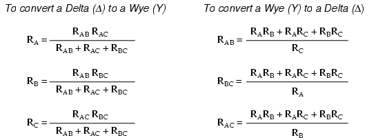
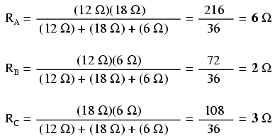
There are several equations used to convert one network to the other:

Δ and Y networks are seen frequently in 3-phase AC power systems (a topic covered in volume II of this book series), but even then they're usually balanced networks (all resistors equal in value) and conversion from one to the other need not involve such complex calculations. When would the average technician ever need to use these equations?

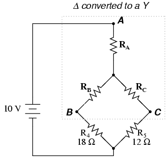
A prime application for Δ-Y conversion is in the solution of unbalanced bridge circuits, such as the one below:

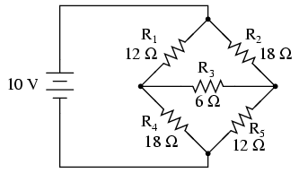
Solution of this circuit with Branch Current or Mesh Current analysis is fairly involved, and neither the Millman nor Superposition Theorems are of any help, since there's only one source of power. We could use Thevenin's or Norton's Theorem, treating R₃ as our load, but what fun would that be?

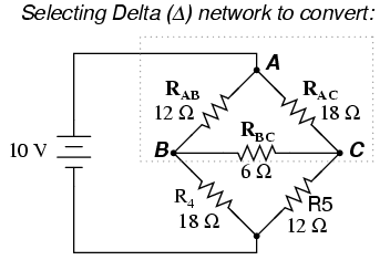
If we were to treat resistors R₁, R₂, and R₃ as being connected in a Δ configuration (R_ab, R_ac, and R_bc, respectively) and generate an equivalent Y network to replace them, we could turn this bridge circuit into a (simpler) series/parallel combination circuit:

After the Δ-Y conversion . . .

If we perform our calculations correctly, the voltages between points A, B, and C will be the same in the converted circuit as in the original circuit, and we can transfer those values back to the original bridge configuration.

Resistors R₄ and R₅, of course, remain the same at 18 Ω and 12 Ω, respectively. Analyzing the circuit now as a series/parallel combination, we arrive at the following figures:

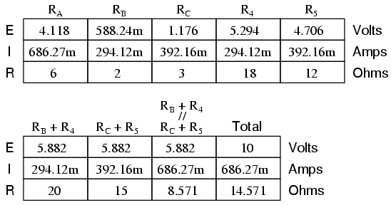
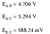
We must use the voltage drops figures from the table above to determine the voltages between points A, B, and C, seeing how the add up (or subtract, as is the case with voltage between points B and C):

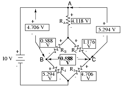
Now that we know these voltages, we can transfer them to the same points A, B, and C in the original bridge circuit:

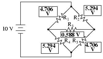
Voltage drops across R₄ and R₅, of course, are exactly the same as they were in the converted circuit.

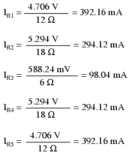
At this point, we could take these voltages and determine resistor currents through the repeated use of Ohm's Law (I=E/R):

A quick simulation with SPICE will serve to verify our work:

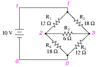
unbalanced bridge circuit   
v1 1 0  
r1 1 2 12       
r2 1 3 18       
r3 2 3 6
r4 2 0 18       
r5 3 0 12       
.dc v1 10 10 1  
.print dc v(1,2) v(1,3) v(2,3) v(2,0) v(3,0)    
.end    

v1            v(1,2)      v(1,3)      v(2,3)      v(2)        v(3)            
1.000E+01     4.706E+00   5.294E+00   5.882E-01   5.294E+00   4.706E+00

The voltage figures, as read from left to right, represent voltage drops across the five respective resistors, R₁ through R₅. I could have shown currents as well, but since that would have required insertion of "dummy" voltage sources in the SPICE netlist, and since we're primarily interested in validating the Δ-Y conversion equations and not Ohm's Law, this will suffice.

• REVIEW:

• "Delta" (Δ) networks are also known as "Pi" (π) networks.

• "Y" networks are also known as "T" networks.

• Δ and Y networks can be converted to their equivalent counterparts with the proper resistance equations. By "equivalent," I mean that the two networks will be electrically identical as measured from the three terminals (A, B, and C).

• A bridge circuit can be simplified to a series/parallel circuit by converting half of it from a Δ to a Y network. After voltage drops between the original three connection points (A, B, and C) have been solved for, those voltages can be transferred back to the original bridge circuit, across those same equivalent points.