Mutual inductance and basic
operation
Suppose we were to wrap a coil of insulated
wire around a loop of ferromagnetic material and energize
this coil with an AC voltage source:
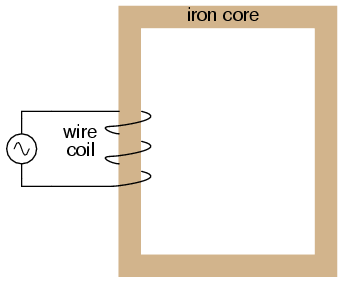
As an inductor, we would expect this
iron-core coil to oppose the applied voltage with its
inductive reactance, limiting current through the coil as
predicted by the equations XL = 2πfL and I=E/X
(or I=E/Z). For the purposes of this example, though, we
need to take a more detailed look at the interactions of
voltage, current, and magnetic flux in the device.
Kirchhoff's voltage law describes how the
algebraic sum of all voltages in a loop must equal zero. In
this example, we could apply this fundamental law of
electricity to describe the respective voltages of the
source and of the inductor coil. Here, as in any one-source,
one-load circuit, the voltage dropped across the load must
equal the voltage supplied by the source, assuming zero
voltage dropped along the resistance of any connecting
wires. In other words, the load (inductor coil) must produce
an opposing voltage equal in magnitude to the source, in
order that it may balance against the source voltage and
produce an algebraic loop voltage sum of zero. From where
does this opposing voltage arise? If the load were a
resistor, the opposing voltage would originate from the
"friction" of electrons flowing through the resistance of
the resistor. With a perfect inductor (no resistance in the
coil wire), the opposing voltage comes from another
mechanism: the reaction to a changing magnetic flux
in the iron core.
Michael Faraday discovered the mathematical
relationship between magnetic flux (Φ) and induced voltage
with this equation:
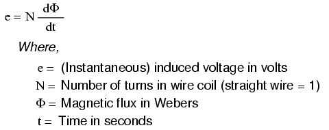
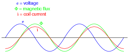
The instantaneous voltage (voltage dropped
at any instant in time) across a wire coil is equal to the
number of turns of that coil around the core (N) multiplied
by the instantaneous rate-of-change in magnetic flux (dΦ/dt)
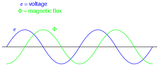
linking with the coil. Graphed, this shows itself as a set
of sine waves (assuming a sinusoidal voltage source), the
flux wave 90o lagging behind the voltage wave:
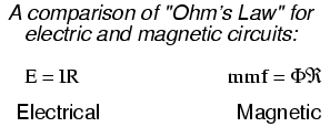
Magnetic flux through a ferromagnetic
material is analogous to current through a conductor: it
must be motivated by some force in order to occur. In
electric circuits, this motivating force is voltage (a.k.a.
electromotive force, or EMF). In magnetic "circuits," this
motivating force is magnetomotive force, or mmf.
Magnetomotive force (mmf) and magnetic flux (Φ) are related
to each other by a property of magnetic materials known as
reluctance (the latter quantity symbolized by a
strange-looking letter "R"):
In our example, the mmf required to produce
this changing magnetic flux (Φ) must be supplied by a
changing current through the coil. Magnetomotive force
generated by an electromagnet coil is equal to the amount of
current through that coil (in amps) multiplied by the number
of turns of that coil around the core (the SI unit for mmf
is the amp-turn). Because the mathematical
relationship between magnetic flux and mmf is directly
proportional, and because the mathematical relationship
between mmf and current is also directly proportional (no
rates-of-change present in either equation), the current
through the coil will be in-phase with the flux wave:
This is why alternating current through an
inductor lags the applied voltage waveform by 90o:
because that is what is required to produce a changing
magnetic flux whose rate-of-change produces an opposing
voltage in-phase with the applied voltage. Due to its
function in providing magnetizing force (mmf) for the core,
this current is sometimes referred to as the magnetizing
current.
It should be mentioned that the current
through an iron-core inductor is not perfectly sinusoidal
(sine-wave shaped), due to the nonlinear B/H magnetization
curve of iron. In fact, if the inductor is cheaply built,
using as little iron as possible, the magnetic flux density
might reach high levels (approaching saturation), resulting
in a magnetizing current waveform that looks something like
this:
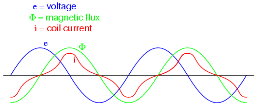
When a ferromagnetic material approaches
magnetic flux saturation, disproportionately greater levels
of magnetic field force (mmf) are required to deliver equal
increases in magnetic field flux (Φ). Because mmf is
proportional to current through the magnetizing coil (mmf =
NI, where "N" is the number of turns of wire in the coil and
"I" is the current through it), the large increases of mmf
required to supply the needed increases in flux results in
large increases in coil current. Thus, coil current
increases dramatically at the peaks in order to maintain a
flux waveform that isn't distorted, accounting for the
bell-shaped half-cycles of the current waveform in the above
plot.
The situation is further complicated by
energy losses within the iron core. The effects of
hysteresis and eddy currents conspire to further distort and
complicate the current waveform, making it even less
sinusoidal and altering its phase to be lagging slightly
less than 90o behind the applied voltage
waveform. This coil current resulting from the sum total of
all magnetic effects in the core (dΦ/dt magnetization plus
hysteresis losses, eddy current losses, etc.) is called the
exciting current. The distortion of an iron-core
inductor's exciting current may be minimized if it is
designed for and operated at very low flux densities.
Generally speaking, this requires a core with large
cross-sectional area, which tends to make the inductor bulky
and expensive. For the sake of simplicity, though, we'll
assume that our example core is far from saturation and free
from all losses, resulting in a perfectly sinusoidal
exciting current.
As we've seen already in the inductors
chapter, having a current waveform 90o out of
phase with the voltage waveform creates a condition where
power is alternately absorbed and returned to the circuit by
the inductor. If the inductor is perfect (no wire
resistance, no magnetic core losses, etc.), it will
dissipate zero power.
Let us now consider the same inductor
device, except this time with a second coil wrapped around
the same iron core. The first coil will be labeled the
primary coil, while the second will be labeled the
secondary:
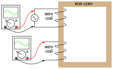
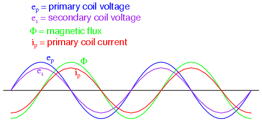
If this secondary coil experiences the same
magnetic flux change as the primary (which it should,
assuming perfect containment of the magnetic flux through
the common core), and has the same number of turns around
the core, a voltage of equal magnitude and phase to the
applied voltage will be induced along its length. In the
following graph, the induced voltage waveform is drawn
slightly smaller than the source voltage waveform simply to
distinguish one from the other:
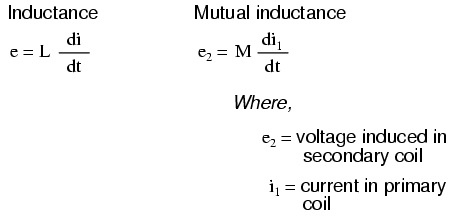
This effect is called mutual inductance:
the induction of a voltage in one coil in response to a
change in current in the other coil. Like normal (self-)
inductance, it is measured in the unit of Henrys, but unlike
normal inductance it is symbolized by the capital letter "M"
rather than the letter "L":
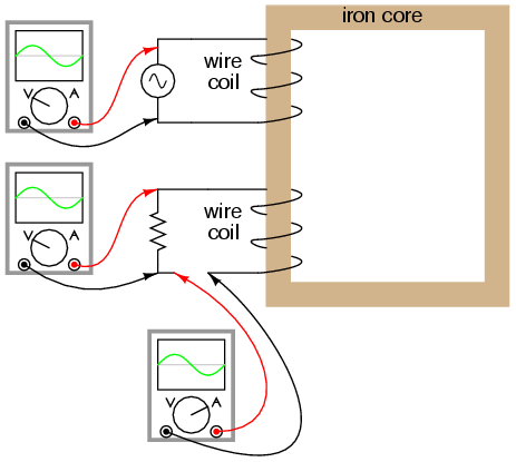
No current will exist in the secondary coil,
since it is open-circuited. However, if we connect a load
resistor to it, an alternating current will go through the
coil, in phase with the induced voltage (because the voltage
across a resistor and the current through it are always
in phase with each other).
At first, one might expect this secondary
coil current to cause additional magnetic flux in the core.
In fact, it does not. If more flux were induced in the core,
it would cause more voltage to be induced voltage in the
primary coil (remember that e = dΦ/dt). This cannot happen,
because the primary coil's induced voltage must remain at
the same magnitude and phase in order to balance with the
applied voltage, in accordance with Kirchhoff's voltage law.
Consequently, the magnetic flux in the core cannot be
affected by secondary coil current. However, what does
change is the amount of mmf in the magnetic circuit.
Magnetomotive force is produced any time
electrons move through a wire. Usually, this mmf is
accompanied by magnetic flux, in accordance with the mmf=ΦR
"magnetic Ohm's Law" equation. In this case, though,
additional flux is not permitted, so the only way the
secondary coil's mmf may exist is if a counteracting mmf is
generated by the primary coil, of equal magnitude and
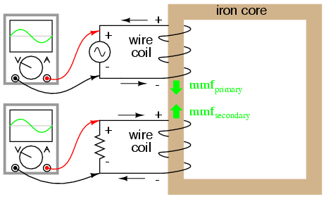
opposite phase. Indeed, this is what happens, an alternating
current forming in the primary coil -- 180o out
of phase with the secondary coil's current -- to generate
this counteracting mmf and prevent additional core flux.
Polarity marks and current direction arrows have been added
to the illustration to clarify phase relations:
If you find this process a bit confusing, do
not worry. Transformer dynamics is a complex subject. What
is important to understand is this: when an AC voltage is
applied to the primary coil, it creates a magnetic flux in
the core, which induces AC voltage in the secondary coil
in-phase with the source voltage. Any current drawn through
the secondary coil to power a load induces a corresponding
current in the primary coil, drawing current from the
source.
Notice how the primary coil is behaving as a
load with respect to the AC voltage source, and how the
secondary coil is behaving as a source with respect to the
resistor. Rather than energy merely being alternately
absorbed and returned the primary coil circuit, energy is
now being coupled to the secondary coil where it is
delivered to a dissipative (energy-consuming) load. As far
as the source "knows," it's directly powering the resistor.
Of course, there is also an additional primary coil current
lagging the applied voltage by 90o, just enough
to magnetize the core to create the necessary voltage for
balancing against the source (the exciting current).
We call this type of device a transformer,
because it transforms electrical energy into magnetic
energy, then back into electrical energy again. Because its
operation depends on electromagnetic induction between two
stationary coils and a magnetic flux of changing magnitude
and "polarity," transformers are necessarily AC devices. Its
schematic symbol looks like two inductors (coils) sharing
the same magnetic core:
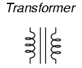
The two inductor coils are easily
distinguished in the above symbol. The pair of vertical
lines represent an iron core common to both inductors. While
many transformers have ferromagnetic core materials, there
are some that do not, their constituent inductors being
magnetically linked together through the air.
The following photograph shows a power
transformer of the type used in gas-discharge lighting.
Here, the two inductor coils can be clearly seen, wound
around an iron core. While most transformer designs enclose
the coils and core in a metal frame for protection, this
particular transformer is open for viewing and so serves its
illustrative purpose well:

Both coils of wire can be seen here with
copper-colored varnish insulation. The top coil is larger
than the bottom coil, having a greater number of "turns"
around the core. In transformers, the inductor coils are
often referred to as windings, in reference to the
manufacturing process where wire is wound around the
core material. As modeled in our initial example, the
powered inductor of a transformer is called the primary
winding, while the unpowered coil is called the secondary
winding.
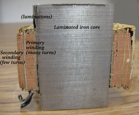
In the next photograph, a transformer is
shown cut in half, exposing the cross-section of the iron
core as well as both windings. Like the transformer shown
previously, this unit also utilizes primary and secondary
windings of differing turn counts. The wire gauge can also
be seen to differ between primary and secondary windings.
The reason for this disparity in wire gauge will be made
clear in the next section of this chapter. Additionally, the
iron core can be seen in this photograph to be made of many
thin sheets (laminations) rather than a solid piece. The
reason for this will also be explained in a later section of
this chapter.
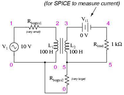
It is easy to demonstrate simple transformer
action using SPICE, setting up the primary and secondary
windings of the simulated transformer as a pair of "mutual"
inductors. The coefficient of magnetic field coupling is
given at the end of the "k" line in the SPICE
circuit description, this example being set very nearly at
perfection (1.000). This coefficient describes how closely
"linked" the two inductors are, magnetically. The better
these two inductors are magnetically coupled, the more
efficient the energy transfer between them should be.
transformer
v1 1 0 ac 10 sin
rbogus1 1 2 1e-12
rbogus2 5 0 9e12
l1 2 0 100
l2 3 5 100
** This line tells SPICE that the two inductors
** l1 and l2 are magnetically "linked" together
k l1 l2 0.999
vi1 3 4 ac 0
rload 4 5 1k
.ac lin 1 60 60
.print ac v(2,0) i(v1)
.print ac v(3,5) i(vi1)
.end
Note: the Rbogus resistors are
required to satisfy certain quirks of SPICE. The first
breaks the otherwise continuous loop between the voltage
source and L1 which would not be permitted by
SPICE. The second provides a path to ground (node 0) from
the secondary circuit, necessary because SPICE cannot
function with any ungrounded circuits.
freq          v(2)        i(v1)
6.000E+01     1.000E+01   9.975E-03   Primary winding
freq          v(3,5)      i(vi1)
6.000E+01     9.962E+00   9.962E-03   Secondary winding
Note that with equal inductances for both
windings (100 Henrys each), the AC voltages and currents are
nearly equal for the two. The difference between primary and
secondary currents is the magnetizing current spoken of
earlier: the 90o lagging current necessary to
magnetize the core. As is seen here, it is usually very
small compared to primary current induced by the load, and
so the primary and secondary currents are almost equal. What
you are seeing here is quite typical of transformer
efficiency. Anything less than 95% efficiency is considered
poor for modern power transformer designs, and this transfer
of power occurs with no moving parts or other components
subject to wear.
If we decrease the load resistance so as to
draw more current with the same amount of voltage, we see
that the current through the primary winding increases in
response. Even though the AC power source is not directly
connected to the load resistance (rather, it is
electromagnetically "coupled"), the amount of current drawn
from the source will be almost the same as the amount of
current that would be drawn if the load were directly
connected to the source. Take a close look at the next two
SPICE simulations, showing what happens with different
values of load resistors:
transformer
v1 1 0 ac 10 sin
rbogus1 1 2 1e-12
rbogus2 5 0 9e12
l1 2 0 100
l2 3 5 100
k l1 l2 0.999
vi1 3 4 ac 0
** Note load resistance value of 200 ohms
rload 4 5 200
.ac lin 1 60 60
.print ac v(2,0) i(v1)
.print ac v(3,5) i(vi1)
.end
freq          v(2)        i(v1)
6.000E+01     1.000E+01   4.679E-02
freq          v(3,5)      i(vi1)
6.000E+01     9.348E+00   4.674E-02
Notice how the primary current closely
follows the secondary current. In our first simulation, both
currents were approximately 10 mA, but now they are both
around 47 mA. In this second simulation, the two currents
are closer to equality, because the magnetizing current
remains the same as before while the load current has
increased. Note also how the secondary voltage has decreased
some with the heavier (greater current) load. Let's try
another simulation with an even lower value of load
resistance (15 Ω):
transformer
v1 1 0 ac 10 sin
rbogus1 1 2 1e-12
rbogus2 5 0 9e12
l1 2 0 100
l2 3 5 100
k l1 l2 0.999
vi1 3 4 ac 0
rload 4 5 15
.ac lin 1 60 60
.print ac v(2,0) i(v1)
.print ac v(3,5) i(vi1)
.end
freq          v(2)        i(v1)
6.000E+01     1.000E+01   1.301E-01
freq          v(3,5)      i(vi1)
6.000E+01     1.950E+00   1.300E-01
Our load current is now 0.13 amps, or 130 mA,
which is substantially higher than the last time. The
primary current is very close to being the same, but notice
how the secondary voltage has fallen well below the primary
voltage (1.95 volts versus 10 volts at the primary). The
reason for this is an imperfection in our transformer
design: because the primary and secondary inductances aren't
perfectly linked (a k factor of 0.999
instead of 1.000) there is "stray" or "leakage"
inductance. In other words, some of the magnetic field isn't
linking with the secondary coil, and thus cannot couple
energy to it:
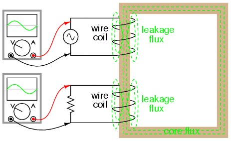
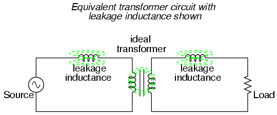
Consequently, this "leakage" flux merely
stores and returns energy to the source circuit via
self-inductance, effectively acting as a series impedance in
both primary and secondary circuits. Voltage gets dropped
across this series impedance, resulting in a reduced load
voltage: voltage across the load "sags" as load current
increases.
If we change the transformer design to have
better magnetic coupling between the primary and secondary
coils, the figures for voltage between primary and secondary
windings will be much closer to equality again:
transformer
v1 1 0 ac 10 sin
rbogus1 1 2 1e-12
rbogus2 5 0 9e12
l1 2 0 100
l2 3 5 100
** Coupling factor = 0.99999 instead of 0.999
k l1 l2 0.99999
vi1 3 4 ac 0
rload 4 5 15
.ac lin 1 60 60
.print ac v(2,0) i(v1)
.print ac v(3,5) i(vi1)
.end
freq          v(2)        i(v1)
6.000E+01     1.000E+01   6.658E-01
freq          v(3,5)      i(vi1)
6.000E+01     9.987E+00   6.658E-01
Here we see that our secondary voltage is
back to being equal with the primary, and the secondary
current is equal to the primary current as well.
Unfortunately, building a real transformer with coupling
this complete is very difficult. A compromise solution is to
design both primary and secondary coils with less
inductance, the strategy being that less inductance overall
leads to less "leakage" inductance to cause trouble, for any
given degree of magnetic coupling inefficiency. This results
in a load voltage that is closer to ideal with the same
(heavy) load and the same coupling factor:
transformer
v1 1 0 ac 10 sin
rbogus1 1 2 1e-12
rbogus2 5 0 9e12
** inductance = 1 henry instead of 100 henrys
l1 2 0 1
l2 3 5 1
k l1 l2 0.999
vi1 3 4 ac 0
rload 4 5 15
.ac lin 1 60 60
.print ac v(2,0) i(v1)
.print ac v(3,5) i(vi1)
.end
freq          v(2)        i(v1)
6.000E+01     1.000E+01   6.664E-01
freq          v(3,5)      i(vi1)
6.000E+01     9.977E+00   6.652E-01
Simply by using primary and secondary coils
of less inductance, the load voltage for this heavy load has
been brought back up to nearly ideal levels (9.977 volts).
At this point, one might ask, "If less inductance is all
that's needed to achieve near-ideal performance under heavy
load, then why worry about coupling efficiency at all? If
it's impossible to build a transformer with perfect
coupling, but easy to design coils with low inductance, then
why not just build all transformers with low-inductance
coils and have excellent efficiency even with poor magnetic
coupling?"
The answer to this question is found in
another simulation: the same low-inductance transformer, but
this time with a lighter load (1 kΩ instead of 15 Ω):
transformer
v1 1 0 ac 10 sin
rbogus1 1 2 1e-12
rbogus2 5 0 9e12
l1 2 0 1
l2 3 5 1
k l1 l2 0.999
vi1 3 4 ac 0
rload 4 5 1k
.ac lin 1 60 60
.print ac v(2,0) i(v1)
.print ac v(3,5) i(vi1)
.end
freq          v(2)        i(v1)
6.000E+01     1.000E+01   2.835E-02
freq          v(3,5)      i(vi1)
6.000E+01     9.990E+00   9.990E-03
With lower winding inductances, the primary
and secondary voltages are closer to being equal, but the
primary and secondary currents are not. In this particular
case, the primary current is 28.35 mA while the secondary
current is only 9.990 mA: almost three times as much current
in the primary as the secondary. Why is this? With less
inductance in the primary winding, there is less inductive
reactance, and consequently a much larger magnetizing
current. A substantial amount of the current through the
primary winding merely works to magnetize the core rather
than transfer useful energy to the secondary winding
and load.
An ideal transformer with identical primary
and secondary windings would manifest equal voltage and
current in both sets of windings for any load condition. In
a perfect world, transformers would transfer electrical
power from primary to secondary as smoothly as though the
load were directly connected to the primary power source,
with no transformer there at all. However, you can see this
ideal goal can only be met if there is perfect
coupling of magnetic flux between primary and secondary
windings. Being that this is impossible to achieve,
transformers must be designed to operate within certain
expected ranges of voltages and loads in order to perform as
close to ideal as possible. For now, the most important
thing to keep in mind is a transformer's basic operating
principle: the transfer of power from the primary to the
secondary circuit via electromagnetic coupling.
-
REVIEW:
-
Mutual inductance is where the
magnetic flux of two or more inductors are "linked" so
that voltage is induced in one coil proportional to the
rate-of-change of current in another.
-
A transformer is a device made of
two or more inductors, one of which is powered by AC,
inducing an AC voltage across the second inductor. If the
second inductor is connected to a load, power will be
electromagnetically coupled from the first inductor's
power source to that load.
-
The powered inductor in a transformer is
called the primary winding. The unpowered inductor
in a transformer is called the secondary winding.
-
Magnetic flux in the core (Φ) lags 90o
behind the source voltage waveform. The current drawn by
the primary coil from the source to produce this flux is
called the magnetizing current, and it also lags
the supply voltage by 90o.
-
Total primary current in an unloaded
transformer is called the exciting current, and is
comprised of magnetizing current plus any additional
current necessary to overcome core losses. It is never
perfectly sinusoidal in a real transformer, but may be
made more so if the transformer is designed and operated
so that magnetic flux density is kept to a minimum.
-
Core flux induces a voltage in any coil
wrapped around the core. The induces voltage(s) are
ideally in phase with the primary winding source voltage
and share the same waveshape.
-
Any current drawn through the secondary
winding by a load will be "reflected" to the primary
winding and drawn from the voltage source, as if the
source were directly powering a similar load.
|
